Making Volcano Plots With ggplot2

One of the, if not the, most common downstream analysis task I'm asked to perform on RNAseq data is to generate the venerable "Volcano Plot." These are kind of the bioinformatics equivalent of saying "Hey! Look how much data I have!" Regardless, they are a pretty good way to quickly summarize an RNAseq experiment. There are now lots of options for generating these visualizations. If you're looking for a plug and play option, the excellent bioconductor package EnhancedVolcano. However, if you are an R tidyverse user you actually already have everything you need to make these plots.

Starting in grad school, I created a library of R and Python snippets that I still reuse. I've continued to update my volcano plot code over time and at this point I actually still reuse that rather than loading in another package. Below, I will share this code and explain the major concepts behind making it. I'm not a software engineer, so it's likely that there are lots of other ways to throw this together.

The Full Function

This function is also available here

library(dplyr)
library(ggplot2)
library(ggrepel)  # For displaying gene labels, if you don't want them you can omit this library

volcplot <- function(data, padj_threshold = 0.05, fc = 1, plot_title = 'Volcano Plot', plot_subtitle = NULL, genelist_vector = NULL, genelist_filter = FALSE) {

  # Set the fold-change thresholds
  neg_log2fc <- -log2(fc)
  pos_log2fc <- log2(fc)

  # Make a dataset for plotting, add the status as a new column
  plot_ready_data <- data %>%
    mutate_at('padj', ~replace(.x, is.na(.x), 1)) %>%
    mutate_at('log2FoldChange', ~replace(.x, is.na(.x), 0)) %>%
    mutate(
      log2fc_threshold = ifelse(log2FoldChange >= pos_log2fc & padj <= padj_threshold, 'up',
                         ifelse(log2FoldChange <= neg_log2fc & padj <= padj_threshold, 'down', 'ns')
        )
    ) %>%
    mutate(hgnc_symbol = replace_na(hgnc_symbol, 'none'))

  if (genelist_filter) {
    plot_ready_data <- plot_ready_data %>% filter(hgnc_symbol %in% genelist_vector)
  }

  if(!is.null(genelist_vector)) {
    plot_ready_data <- plot_ready_data %>% mutate(hgnc_symbol = ifelse(hgnc_symbol %in% genelist_vector & padj < padj_threshold & log2fc_threshold != 'ns', hgnc_symbol, ''))
  }

  # Get the number of up, down, and unchanged genes
  up_genes <- plot_ready_data %>% filter(log2fc_threshold == 'up') %>% nrow()
  down_genes <- plot_ready_data %>% filter(log2fc_threshold == 'down') %>% nrow()
  unchanged_genes <- plot_ready_data %>% filter(log2fc_threshold == 'ns') %>% nrow()

  # Make the labels for the legend
  legend_labels <- c(
      str_c('Up: ', up_genes),
      str_c('NS: ', unchanged_genes),
      str_c('Down: ', down_genes)
  )

  # Set the x axis limits, rounded to the next even number
  x_axis_limits <- DescTools::RoundTo(
    max(abs(plot_ready_data$log2FoldChange)),
    2,
    ceiling
  )

  # Set the plot colors
  plot_colors <- c(
      'up' = 'firebrick1',
      'ns' = 'gray',
      'down' = 'dodgerblue1'
  )


  # Make the plot, these options are a reasonable strting point
  plot <- ggplot(plot_ready_data) +
    geom_point(
      alpha = 0.25,
      size = 1.5
    ) +
    aes(
      x = log2FoldChange,
      y = -log10(padj),
      color = log2fc_threshold,
      label = hgnc_symbol
    ) +
    geom_vline(
      xintercept = c(neg_log2fc, pos_log2fc),
      linetype = 'dashed'
    ) +
    geom_hline(
      yintercept = -log10(padj_threshold),
      linetype = 'dashed'
    ) +
    scale_x_continuous(
      'log2(FC)',
      limits = c(-x_axis_limits, x_axis_limits)
    ) +
    scale_color_manual(
      values = plot_colors,
      labels = legend_labels
      ) +
    labs(
      color = str_c(fc, '-fold, padj ≤', padj_threshold),
      title = plot_title,
      subtitle = plot_subtitle
    ) +
    theme_bw(base_size = 24) +
    theme(
      aspect.ratio = 1,
      axis.text = element_text(color = 'black'),
      legend.margin = margin(0, 0, 0, 0),
      legend.box.margin = margin(0, 0, 0, 0),  # Reduces dead area around legend
      legend.spacing.x = unit(0.2, 'cm')
    )

    # Add gene labels if needed
    if (!is.null(genelist_vector)) {
        plot <- plot +
        geom_label_repel(
          size = 6,
          force = 0.1,
          max.overlaps = 100000,
          nudge_x = 1,
          segment.color = 'black',
          min.segment.length = 0,
          show.legend = FALSE
        )
    }
    plot
}

Yes, this is rather long, but it's actually fairly straightforward to understand. Hopefully the comments help.

But What Does This Look Like?

Here's an example of a typical volcano plot this generates:

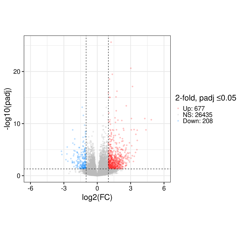
There are lots of places to customize, of course, since it's just a normal ggplot2 object.

How Is The Input Data Formatted?

This function works with DESeq2 output results as a data frame, but requires a bit of reformatting. So, you can get there like this:

deseq_results <- as.data.frame(deseq2_results) %>%
    rownamnes_to_column(var = 'ensembl_id') %>%
    left_join({ensembl_id_hgnc_symbol})

I typically work with ensembl gene IDs as a ground truth identifier for genes, and also include gene symbols as a more human readable identifier. Since I'm primarily working with human cell lines at the moment there needs to be a column in your dataset called "hgnc_symbol," according to the design of the volcano plot function. We achieve this by left_join() with an additional dataframe that consists of only two columns, "ensembl_id" and "hgnc_symbol." If you do work in mice, plants, etc. you can change all references to that column to suit your needs both here and in the plotting function.

Brief Explanation

You can think of this function doing things in a few discrete steps:

1. Set the fold chance thresholds for the plot based on what you provide for the variable fc, which defaults to 1 (no threshold).
2. Set NAs in the padj column to 1 and in the log2FoldChange column to 0. Create a new variable with the gene's differential expression status (up, down, not significant).
3. Filter the dataset on a list of hgnc symbols you supply (optional).
4. Remove gene symbol labels if not differentially expressed and not a member of a list supplied when invoking the function (optional).
5. Get the number of genes which are significantly up and down, and the number which are not significant for the legend.
6. Create the legend labels based on number of differentially expressed genes.
7. Set the X axis limits based on rounding to the next multiple of 2 (because log base 2) of the absolute value of the max in the log2FoldChange column.
8. Set the colors for the plot, defaults can be easily changed but I like them.
9. Build the ggplot object, simply using geom_point() and some vertical/horizontal lines based on your fold change and padj thresholds.
10. Add labels to points based on hgnc_symbol (optional).

Some Gotchas

DESeq2 sets padj and log2foldchange to NA for many reasons. This may be because of the expression level and filtering out low-expressing genes prior to statistical testing. It may also be due to lack of replicates and too much variability. Regardless, it's something of a philosophical question as to whether you want these genes to show up in the "not significant" category or whether you should simply not include them in the results at all. At this point, I lean toward setting their p values to 1 and log fold changes to 0. This way, such genes end up in the "not significant" category. My reasoning, this heads off question about why the number of genes in each category may not add up to the number in the annotation set across comparisons. Now those genes which are significantly up, down, and not significant always add up to the same number assuming that you're using the same annotations.

Why Not Just Use EnhancedVolcano?

Honestly, there isn't really a good reason not to. However, I already had this code on-hand and therefore I find it pretty easy to just run this on the reg. If you're learning ggplot2 and the tidyverse I think this is a good way to learn with a real example.